Anomaly Detection Using an Autoencoder

If you’re running this in Colab, make sure to save a copy of the notebook in Google Drive to save your changes.

The datasets used in this notebook

To detect and visualise hidden anomalies, we will be using the open-source Numenta Anolmaly Benchmark (NAB) dataset. The raw versions of the art_daily_small_noise.csv and art_daily_jump.csv datasets are available here and here, respectively. For a deeper understanding of the code cells, the curious reader should familiarise themselves with Python and the NumPy, Matplotliband Pandas libraries, and possibly the TensorFlow platform.

Setup

# If you're running this notebook, uncomment the code in this cell to install the required packages.
# ! pip install numpy
# ! pip install pandas
# ! pip install tensorflow
# ! pip install matplotlib

import numpy as np
import pandas as pd
from tensorflow import keras
from tensorflow.keras import layers
from matplotlib import pyplot as plt

Load the data

In addition to the NAB dataset, we will use the art_daily_small_noise.csv file for training and the art_daily_jump.csv file for testing our model. Note that the terms ‘test set’ and ‘validation set’ will be used interchangably, and that all three datasets used in this demonstration consist of synthetic data. To see how synthetic datasets are generated and why they are useful in data science, take a look at the complementary ‘Linear Regression and Coulomb’s Law’ section. The simplicity of these datasets allows us to demonstrate anomaly detection effectively.

The following commands will ensure our datasets are imported and converted from CSV format to a Pandas DataFrame to faciliate further analysis:

master_url_root = "https://raw.githubusercontent.com/numenta/NAB/master/data/"

df_small_noise_url_suffix = "artificialNoAnomaly/art_daily_small_noise.csv"
df_small_noise_url = master_url_root + df_small_noise_url_suffix
df_small_noise = pd.read_csv(
    df_small_noise_url, parse_dates=True, index_col="timestamp"
)

df_daily_jumpsup_url_suffix = "artificialWithAnomaly/art_daily_jumpsup.csv"
df_daily_jumpsup_url = master_url_root + df_daily_jumpsup_url_suffix
df_daily_jumpsup = pd.read_csv(
    df_daily_jumpsup_url, parse_dates=True, index_col="timestamp"
)

Quick look at the data

The artificial timeseries data we will be working with are ordered, timestamped, single-valued metrics, with labeled periods of anomalous behaviour.

Run the commands below for a brief overview of what our training and test sets look like:

print(df_small_noise.head())
print(df_daily_jumpsup.head())

                         value
timestamp
2014-04-01 00:00:00  18.324919
2014-04-01 00:05:00  21.970327
2014-04-01 00:10:00  18.624806
2014-04-01 00:15:00  21.953684
2014-04-01 00:20:00  21.909120
                         value
timestamp
2014-04-01 00:00:00  19.761252
2014-04-01 00:05:00  20.500833
2014-04-01 00:10:00  19.961641
2014-04-01 00:15:00  21.490266
2014-04-01 00:20:00  20.187739

Visualise the data

Timeseries data without anomalies

Our main task during the training stage will be to train the model and establish a suitable benchmark for an anomaly. How accurate is our model and what is the threshold for classifying an abnormal datapoint?

Here is the data we will use for training:

fig, ax = plt.subplots()
df_small_noise.plot(legend=False, ax=ax)
plt.xlabel("Timestamp")
plt.title("Training data")
plt.show()

Timeseries data with anomalies

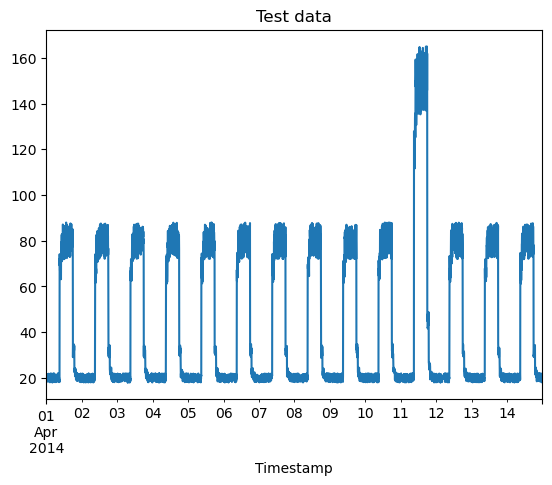
To test the autoencoder after the training stage, we want to see whether the spike in our artificial test data will be successfully detected as an anomaly. In practice, this could be a much smaller discrepancy embedded in a noisy astronomical dataset, which we would expect our model to be able to detect and bring to our attention.

Here is our training data visualised:

fig, ax = plt.subplots()
df_daily_jumpsup.plot(legend=False, ax=ax)
plt.xlabel("Timestamp")
plt.title("Test data")
plt.show()

Prepare training data

First, isolate the values of interest from the training dataset and normalise the value column. Normalisation is done by subtracting the training_mean from each value datapoint and dividing by the training_std. We have a value entry every 5 minutes for 14 days, giving us a total of 4032 samples.

# Normalise and save the mean and standard deviation we get for normalising test data.
training_mean = df_small_noise.mean()
training_std = df_small_noise.std()
df_training_value = (df_small_noise - training_mean) / training_std

# Output the normalised training data.
print(df_training_value.head())

# Output the number of samples.
print("\nNumber of training samples:", len(df_training_value))

                        value
timestamp
2014-04-01 00:00:00 -0.858829
2014-04-01 00:05:00 -0.728993
2014-04-01 00:10:00 -0.848148
2014-04-01 00:15:00 -0.729586
2014-04-01 00:20:00 -0.731173

Number of training samples: 4032

Create sequences

Create a series of sequences by combining TIME_STEPS contiguous data values from the training data, changing the starting index with each iteration:

TIME_STEPS = 288

# Generated training sequences for use in the model.
def create_sequences(values, time_steps=TIME_STEPS):
    output = []
    for i in range(len(values) - time_steps + 1):
        output.append(values[i:(i + time_steps)])
    return np.stack(output)

x_train = create_sequences(df_training_value.values)

# Display the first 4 sequences.
print(x_train[0:4])
print("\nTraining input shape: ", x_train.shape)

[[[-0.85882857]
  [-0.72899302]
  [-0.84814772]
  ...
  [-0.86453747]
  [-0.81250829]
  [-0.79671155]]

 [[-0.72899302]
  [-0.84814772]
  [-0.72958579]
  ...
  [-0.81250829]
  [-0.79671155]
  [-0.78767946]]

 [[-0.84814772]
  [-0.72958579]
  [-0.731173  ]
  ...
  [-0.79671155]
  [-0.78767946]
  [-0.73706287]]

 [[-0.72958579]
  [-0.731173  ]
  [-0.75730984]
  ...
  [-0.78767946]
  [-0.73706287]
  [-0.77462891]]]

Training input shape:  (3745, 288, 1)

Build a model

We will build a convolutional reconstruction autoencoder model, which will take an input of shape (batch_size, sequence_length, num_features) and return an output of the same shape. In this case, sequence_length = 288 and num_features = 1.

model = keras.Sequential(
    [
        layers.Input(shape=(x_train.shape[1], x_train.shape[2])),
        layers.Conv1D(
            filters=32, kernel_size=7, padding="same", strides=2, activation="relu"
        ),
        layers.Dropout(rate=0.2),
        layers.Conv1D(
            filters=16, kernel_size=7, padding="same", strides=2, activation="relu"
        ),
        layers.Conv1DTranspose(
            filters=16, kernel_size=7, padding="same", strides=2, activation="relu"
        ),
        layers.Dropout(rate=0.2),
        layers.Conv1DTranspose(
            filters=32, kernel_size=7, padding="same", strides=2, activation="relu"
        ),
        layers.Conv1DTranspose(filters=1, kernel_size=7, padding="same"),
    ]
)

model.compile(optimizer=keras.optimizers.Adam(learning_rate=0.001), loss="mse")
model.summary()

Model: "sequential"
_________________________________________________________________
 Layer (type)                Output Shape              Param #
=================================================================
 conv1d (Conv1D)             (None, 144, 32)           256

 dropout (Dropout)           (None, 144, 32)           0

 conv1d_1 (Conv1D)           (None, 72, 16)            3600

 conv1d_transpose (Conv1DTra  (None, 144, 16)          1808
 nspose)

 dropout_1 (Dropout)         (None, 144, 16)           0

 conv1d_transpose_1 (Conv1DT  (None, 288, 32)          3616
 ranspose)

 conv1d_transpose_2 (Conv1DT  (None, 288, 1)           225
 ranspose)

=================================================================
Total params: 9,505
Trainable params: 9,505
Non-trainable params: 0
_________________________________________________________________

Train the model

Having created the model, we will now supply it with the training data. Note that x_train is used as both the input and the target since this is a reconstruction model.

history = model.fit(
    x_train,
    x_train,
    epochs=50,
    batch_size=128,
    validation_split=0.1,
    callbacks=[
        keras.callbacks.EarlyStopping(monitor="val_loss", patience=5, mode="min")
    ],
)

Epoch 1/50
27/27 [==============================] - 3s 59ms/step - loss: 0.4390 - val_loss: 0.0529
Epoch 2/50
27/27 [==============================] - 1s 43ms/step - loss: 0.0790 - val_loss: 0.0457
Epoch 3/50
27/27 [==============================] - 1s 42ms/step - loss: 0.0608 - val_loss: 0.0390
Epoch 4/50
27/27 [==============================] - 1s 46ms/step - loss: 0.0530 - val_loss: 0.0343
Epoch 5/50
27/27 [==============================] - 1s 48ms/step - loss: 0.0463 - val_loss: 0.0304
Epoch 6/50
27/27 [==============================] - 1s 51ms/step - loss: 0.0402 - val_loss: 0.0252
Epoch 7/50
27/27 [==============================] - 1s 49ms/step - loss: 0.0348 - val_loss: 0.0216
Epoch 8/50
27/27 [==============================] - 1s 49ms/step - loss: 0.0312 - val_loss: 0.0198
Epoch 9/50
27/27 [==============================] - 1s 47ms/step - loss: 0.0287 - val_loss: 0.0188
Epoch 10/50
27/27 [==============================] - 1s 48ms/step - loss: 0.0266 - val_loss: 0.0184
Epoch 11/50
27/27 [==============================] - 1s 47ms/step - loss: 0.0250 - val_loss: 0.0189
Epoch 12/50
27/27 [==============================] - 1s 50ms/step - loss: 0.0237 - val_loss: 0.0183
Epoch 13/50
27/27 [==============================] - 1s 49ms/step - loss: 0.0225 - val_loss: 0.0178
Epoch 14/50
27/27 [==============================] - 1s 46ms/step - loss: 0.0216 - val_loss: 0.0190
Epoch 15/50
27/27 [==============================] - 1s 46ms/step - loss: 0.0207 - val_loss: 0.0183
Epoch 16/50
27/27 [==============================] - 1s 45ms/step - loss: 0.0199 - val_loss: 0.0181
Epoch 17/50
27/27 [==============================] - 1s 48ms/step - loss: 0.0192 - val_loss: 0.0178
Epoch 18/50
27/27 [==============================] - 1s 46ms/step - loss: 0.0186 - val_loss: 0.0183
Epoch 19/50
27/27 [==============================] - 1s 46ms/step - loss: 0.0180 - val_loss: 0.0176
Epoch 20/50
27/27 [==============================] - 1s 47ms/step - loss: 0.0175 - val_loss: 0.0166
Epoch 21/50
27/27 [==============================] - 1s 51ms/step - loss: 0.0170 - val_loss: 0.0173
Epoch 22/50
27/27 [==============================] - 1s 51ms/step - loss: 0.0166 - val_loss: 0.0160
Epoch 23/50
27/27 [==============================] - 1s 49ms/step - loss: 0.0162 - val_loss: 0.0163
Epoch 24/50
27/27 [==============================] - 1s 46ms/step - loss: 0.0158 - val_loss: 0.0158
Epoch 25/50
27/27 [==============================] - 1s 50ms/step - loss: 0.0154 - val_loss: 0.0157
Epoch 26/50
27/27 [==============================] - 1s 47ms/step - loss: 0.0151 - val_loss: 0.0148
Epoch 27/50
27/27 [==============================] - 1s 48ms/step - loss: 0.0147 - val_loss: 0.0141
Epoch 28/50
27/27 [==============================] - 1s 45ms/step - loss: 0.0144 - val_loss: 0.0137
Epoch 29/50
27/27 [==============================] - 1s 48ms/step - loss: 0.0141 - val_loss: 0.0129
Epoch 30/50
27/27 [==============================] - 1s 46ms/step - loss: 0.0137 - val_loss: 0.0131
Epoch 31/50
27/27 [==============================] - 1s 47ms/step - loss: 0.0133 - val_loss: 0.0126
Epoch 32/50
27/27 [==============================] - 1s 47ms/step - loss: 0.0130 - val_loss: 0.0121
Epoch 33/50
27/27 [==============================] - 1s 46ms/step - loss: 0.0126 - val_loss: 0.0112
Epoch 34/50
27/27 [==============================] - 1s 55ms/step - loss: 0.0123 - val_loss: 0.0118
Epoch 35/50
27/27 [==============================] - 1s 50ms/step - loss: 0.0119 - val_loss: 0.0103
Epoch 36/50
27/27 [==============================] - 1s 45ms/step - loss: 0.0116 - val_loss: 0.0108
Epoch 37/50
27/27 [==============================] - 1s 52ms/step - loss: 0.0112 - val_loss: 0.0104
Epoch 38/50
27/27 [==============================] - 1s 47ms/step - loss: 0.0110 - val_loss: 0.0100
Epoch 39/50
27/27 [==============================] - 1s 47ms/step - loss: 0.0106 - val_loss: 0.0095
Epoch 40/50
27/27 [==============================] - 1s 51ms/step - loss: 0.0103 - val_loss: 0.0092
Epoch 41/50
27/27 [==============================] - 1s 46ms/step - loss: 0.0100 - val_loss: 0.0090
Epoch 42/50
27/27 [==============================] - 1s 49ms/step - loss: 0.0097 - val_loss: 0.0090
Epoch 43/50
27/27 [==============================] - 1s 51ms/step - loss: 0.0095 - val_loss: 0.0087
Epoch 44/50
27/27 [==============================] - 1s 45ms/step - loss: 0.0092 - val_loss: 0.0082
Epoch 45/50
27/27 [==============================] - 1s 43ms/step - loss: 0.0090 - val_loss: 0.0084
Epoch 46/50
27/27 [==============================] - 1s 45ms/step - loss: 0.0087 - val_loss: 0.0078
Epoch 47/50
27/27 [==============================] - 1s 42ms/step - loss: 0.0085 - val_loss: 0.0079
Epoch 48/50
27/27 [==============================] - 1s 45ms/step - loss: 0.0083 - val_loss: 0.0074
Epoch 49/50
27/27 [==============================] - 1s 42ms/step - loss: 0.0081 - val_loss: 0.0067
Epoch 50/50
27/27 [==============================] - 1s 48ms/step - loss: 0.0079 - val_loss: 0.0068

Let’s plot the training loss and validation loss to see how the model performed. For an optimal fit, we would expect to see the two curves decrease and eventually stabilise at a specific value.

plt.plot(history.history["loss"], label="Training Loss")
plt.plot(history.history["val_loss"], label="Validation Loss")
plt.xlabel("Epochs")
plt.ylabel("Loss")
plt.legend()
plt.show()

Detecting anomalies

We will detect anomalies by determining how well our model can reconstruct the input data.

1. Find MAE loss on the training samples.

2. Find the maximum MAE loss value. This is the worst our model has performed trying to reconstruct a sample. We will make this the threshold for anomaly detection.

3. If the reconstruction loss for a sample is greater than this threshold value, we can infer that the model is seeing a pattern that it isn’t familiar with and will tag this sample as an anomaly.

# Get training MAE loss.
x_train_pred = model.predict(x_train)
train_mae_loss = np.mean(np.abs(x_train_pred - x_train), axis=1)

plt.hist(train_mae_loss, bins=50)
plt.xlabel("Train MAE loss")
plt.ylabel("Number of samples")
plt.title("Training MAE loss")
plt.show()

# Get reconstruction loss threshold.
threshold = np.max(train_mae_loss)
print("Reconstruction error threshold: ", threshold)

118/118 [==============================] - 2s 11ms/step

Reconstruction error threshold:  0.07229737499847969

Compare reconstruction

To see how the model has reconstructed the first sample, run the code below. This sample consists of the contiguous 288 timesteps starting at Day 1 of our training dataset.

# Check how the first sequence has been learned.
plt.plot(x_train[0], label="Training data")
plt.plot(x_train_pred[0], label="Reconstruction")
plt.legend()
plt.show()

Prepare test data

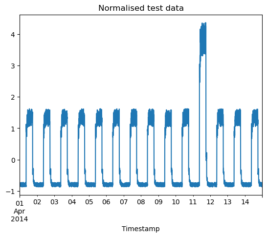
Next, we will test the model on our validation dataset. The code below will output the indices of the anomalous datapoints, as well as visualise the normalised validation dataset and plot a histogram showing the distribution of MAE loss.

df_test_value = (df_daily_jumpsup - training_mean) / training_std
fig, ax = plt.subplots()
df_test_value.plot(legend=False, ax=ax)
plt.xlabel("Timestamp")
plt.title("Normalised test data")
plt.show()

# Create sequences from test values.
x_test = create_sequences(df_test_value.values)
print("Test input shape: ", x_test.shape)

# Calculate the test MAE loss.
x_test_pred = model.predict(x_test)
test_mae_loss = np.mean(np.abs(x_test_pred - x_test), axis=1)
test_mae_loss = test_mae_loss.reshape((-1))

plt.hist(test_mae_loss, bins=50)
plt.xlabel("Test MAE loss")
plt.ylabel("Number of samples")
plt.title("Test MAE loss")
plt.show()

# Detect all the samples which are anomalies.
anomalies = test_mae_loss > threshold
print("Number of anomaly samples: ", np.sum(anomalies))
print("Indices of anomaly samples: ", np.where(anomalies))

Test input shape:  (3745, 288, 1)
118/118 [==============================] - 1s 11ms/step

Number of anomaly samples:  414
Indices of anomaly samples:  (array([ 217,  792,  793,  794,  795, 1649, 1657, 1658, 1945, 2518, 2519,
       2521, 2522, 2523, 2698, 2699, 2701, 2702, 2703, 2704, 2705, 2706,
       2707, 2708, 2709, 2710, 2711, 2712, 2713, 2714, 2715, 2716, 2717,
       2718, 2719, 2720, 2721, 2722, 2723, 2724, 2725, 2726, 2727, 2728,
       2729, 2730, 2731, 2732, 2733, 2734, 2735, 2736, 2737, 2738, 2739,
       2740, 2741, 2742, 2743, 2744, 2745, 2746, 2747, 2748, 2749, 2750,
       2751, 2752, 2753, 2754, 2755, 2756, 2757, 2758, 2759, 2760, 2761,
       2762, 2763, 2764, 2765, 2766, 2767, 2768, 2769, 2770, 2771, 2772,
       2773, 2774, 2775, 2776, 2777, 2778, 2779, 2780, 2781, 2782, 2783,
       2784, 2785, 2786, 2787, 2788, 2789, 2790, 2791, 2792, 2793, 2794,
       2795, 2796, 2797, 2798, 2799, 2800, 2801, 2802, 2803, 2804, 2805,
       2806, 2807, 2808, 2809, 2810, 2811, 2812, 2813, 2814, 2815, 2816,
       2817, 2818, 2819, 2820, 2821, 2822, 2823, 2824, 2825, 2826, 2827,
       2828, 2829, 2830, 2831, 2832, 2833, 2834, 2835, 2836, 2837, 2838,
       2839, 2840, 2841, 2842, 2843, 2844, 2845, 2846, 2847, 2848, 2849,
       2850, 2851, 2852, 2853, 2854, 2855, 2856, 2857, 2858, 2859, 2860,
       2861, 2862, 2863, 2864, 2865, 2866, 2867, 2868, 2869, 2870, 2871,
       2872, 2873, 2874, 2875, 2876, 2877, 2878, 2879, 2880, 2881, 2882,
       2883, 2884, 2885, 2886, 2887, 2888, 2889, 2890, 2891, 2892, 2893,
       2894, 2895, 2896, 2897, 2898, 2899, 2900, 2901, 2902, 2903, 2904,
       2905, 2906, 2907, 2908, 2909, 2910, 2911, 2912, 2913, 2914, 2915,
       2916, 2917, 2918, 2919, 2920, 2921, 2922, 2923, 2924, 2925, 2926,
       2927, 2928, 2929, 2930, 2931, 2932, 2933, 2934, 2935, 2936, 2937,
       2938, 2939, 2940, 2941, 2942, 2943, 2944, 2945, 2946, 2947, 2948,
       2949, 2950, 2951, 2952, 2953, 2954, 2955, 2956, 2957, 2958, 2959,
       2960, 2961, 2962, 2963, 2964, 2965, 2966, 2967, 2968, 2969, 2970,
       2971, 2972, 2973, 2974, 2975, 2976, 2977, 2978, 2979, 2980, 2981,
       2982, 2983, 2984, 2985, 2986, 2987, 2988, 2989, 2990, 2991, 2992,
       2993, 2994, 2995, 2996, 2997, 2998, 2999, 3000, 3001, 3002, 3003,
       3004, 3005, 3006, 3007, 3008, 3009, 3010, 3011, 3012, 3013, 3014,
       3015, 3016, 3017, 3018, 3019, 3020, 3021, 3022, 3023, 3024, 3025,
       3026, 3027, 3028, 3029, 3030, 3031, 3032, 3033, 3034, 3035, 3036,
       3037, 3038, 3039, 3040, 3041, 3042, 3043, 3044, 3045, 3046, 3047,
       3048, 3049, 3050, 3051, 3052, 3053, 3054, 3055, 3056, 3057, 3058,
       3059, 3060, 3061, 3062, 3063, 3064, 3065, 3066, 3067, 3068, 3069,
       3070, 3071, 3072, 3073, 3074, 3075, 3076, 3077, 3078, 3079, 3080,
       3081, 3082, 3083, 3084, 3085, 3086, 3087, 3088, 3089, 3090, 3091,
       3092, 3093, 3094, 3095, 3097, 3099, 3100], dtype=int64),)

Plot anomalies

Having identified the anomalous data, we can now find the corresponding timestamps from the original test data using the following method:

Suppose a simple case where time_steps = 3. For 10 training values, x_train would be:

0, 1, 2
1, 2, 3
2, 3, 4
3, 4, 5
4, 5, 6
5, 6, 7
6, 7, 8
7, 8, 9

All points except the initial and final time_steps - 1 values will appear in a total of time_steps samples. So, if we know that the samples [(3, 4, 5), (4, 5, 6), (5, 6, 7)] are anomalies, we can conclude that the datapoint 5 is an anomaly.

Identify the timestamps values at which the anomalies occur and compile them into a list:

# Datapoint [i] is an anomaly if samples [(i - time_steps + 1) to (i)] are anomalies.
anomalous_data_indices = []
for data_idx in range(TIME_STEPS - 1, len(df_test_value) - TIME_STEPS + 1):
    if np.all(anomalies[data_idx - TIME_STEPS + 1 : data_idx]):
        anomalous_data_indices.append(data_idx)

Finally, let’s overlay the anomalies we found on the original test dataset plot.

df_subset = df_daily_jumpsup.iloc[anomalous_data_indices]
fig, ax = plt.subplots()
df_daily_jumpsup.plot(legend=False, ax=ax)
df_subset.plot(legend=False, ax=ax)
plt.xlabel("Timestamp")
plt.title("Test data with anomalies")

plt.show()

Conclusions

At this point, hopefully it has become clear why visualising and graphing data is an essential component of data science. Compare looking at the indices of the anomalies to looking at the same points superposed on the original plot. While the former is a block of seemingly arbitrary numerical jargon, the latter provides a much more clear overview of this information such that it can be understood from a glance. Not only does this concentrate our attention on the most interesting part of the data, but these insights can be communicated easily to other physicists and laymen. One can also appreciate how delegating this task to a machine saves astronomers such as Jocelyn Bell Burnell from ploughing through months of observational data.

References

Autoencoder model and NAB dataset:

• https://huggingface.co/keras-io/timeseries-anomaly-detection

• https://www.kaggle.com/datasets/boltzmannbrain/nab

Jocelyn Bell Burnell and pulsars:

• https://www.cam.ac.uk/stories/journeysofdiscovery-pulsars

• https://starchild.gsfc.nasa.gov/docs/StarChild/whos_who_level2/bell.html

If you wish to get an overview of the remaining topics in this course, click the button below.